Introduction: Unlocking the World of Data
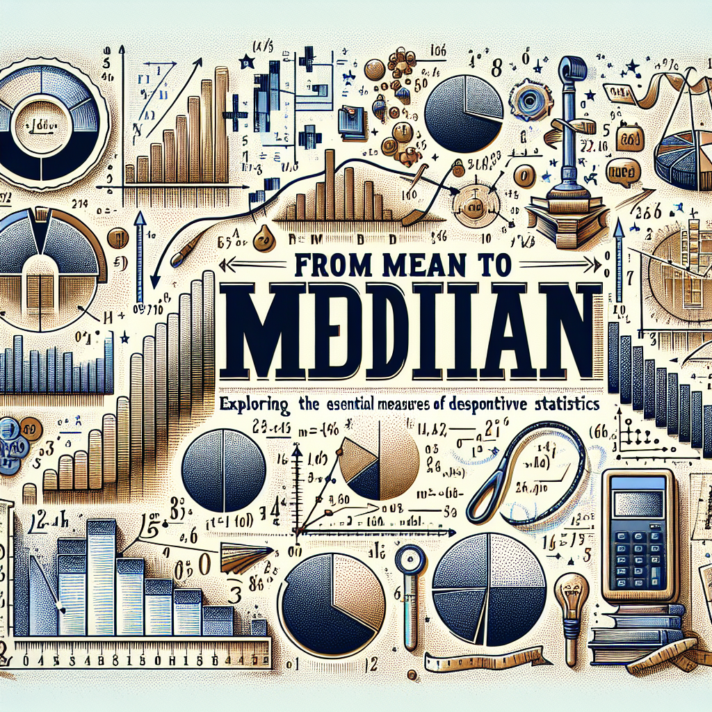
In today’s data-driven society, understanding how to interpret and utilize information is crucial. Whether you are a business executive analyzing sales figures, a student grappling with class averages, or a data scientist sifting through complex datasets, the importance of descriptive statistics cannot be overstated. Among these statistics, two of the most frequently discussed measures are the mean and the median. From Mean to Median: Exploring the Essential Measures of Descriptive Statistics not only reveals the distinction between these two fundamental concepts but also equips you with the tools to apply them effectively in real-world scenarios.
Understanding Descriptive Statistics
Descriptive statistics are metrics that summarize and provide insights into datasets. They serve as the backbone of data analysis, allowing us to condense complex information into understandable formats. The primary measures of descriptive statistics include:
- Mean (Average)
- Median (Middle Value)
- Mode (Most Frequent Value)
- Range (Difference Between Maximum and Minimum)
- Standard Deviation (Measure of Dispersion)
Each of these measures serves a unique purpose and has its own strengths and weaknesses. In this article, we will delve deeper into the mean and median, highlighting their applications, advantages, and limitations.
The Mean: Understanding the Average
What is the Mean?
The mean, often referred to as the average, is calculated by adding all numbers in a dataset and dividing by the count of those numbers. For example, if the scores of a group of students are 90, 80, 70, and 60, the mean would be:
[
\text{Mean} = \frac{90 + 80 + 70 + 60}{4} = \frac{300}{4} = 75
]
Advantages of the Mean
- Simplicity: The calculation is straightforward and easy to understand.
- Usefulness: It considers all numbers in the dataset, providing a holistic view.
Limitations of the Mean
- Sensitivity to Outliers: The mean can be skewed by extreme values. For example, if one of the students scored 20 instead of 60, the mean drops dramatically:
[
\text{New Mean} = \frac{90 + 80 + 70 + 20}{4} = \frac{260}{4} = 65
]
- Not Always Representative: In datasets with significant variability or skewness, the mean may not accurately depict a "typical" value.
Case Study: Salaries in a Company
Consider a technology firm where five employees earn $50,000, $52,000, $53,000, $54,000, and $1,000,000. The mean salary would be computed as follows:
[
\text{Mean Salary} = \frac{50,000 + 52,000 + 53,000 + 54,000 + 1,000,000}{5} = \frac{1,209,000}{5} = 241,800
]
In this case, the mean suggests that the average salary is significantly high due to the outlier, making the median a better measure of central tendency.
The Median: The Middle Ground
What is the Median?
The median is the middle value of a dataset when arranged in ascending or descending order. For the earlier example of student scores, when sorted as 60, 70, 80, 90, the median is:
- Odd-number of observations: The middle score is 75.
- Even-number of observations: The median is the average of the two middle values.
Advantages of the Median
Robustness Against Outliers: The median is less affected by extreme values. It effectively represents the "central" point of a dataset.
- Independency: It provides a better sense of the actual distribution, especially with skewed data.
Limitations of the Median
Ignoring All Data Points: The median only considers the middle value(s), potentially overlooking essential information from the entire dataset.
- Difficult to Calculate with Large Datasets: Finding the median in extensive datasets can become cumbersome if you don’t use computational tools.
Case Study: Home Prices
Consider a neighborhood where home prices are as follows: $200,000, $210,000, $220,000, $250,000, and $1,000,000. The median is:
- Arranging the data: $200,000, $210,000, $220,000, $250,000, $1,000,000
- The median here is $220,000.
In this instance, the median price of $220,000 is much more reflective of the market than the mean price, which would be significantly affected by the $1,000,000 home.
Exploring Variability: Mode, Range, and Standard Deviation
While this article focuses predominantly on the mean and median, it’s essential to understand other measures like the mode, range, and standard deviation, as they contribute valuable insights.
Mode
The mode is the value that appears most frequently in a dataset. Understanding the mode can enhance data interpretation, especially in categorical data analysis.
Range
The range gives the difference between the highest and lowest values. It gives a quick understanding of the spread of the data.
- Example: For the dataset $200,000, $210,000, $220,000, $250,000, and $1,000,000, the range is:
[
\text{Range} = 1,000,000 – 200,000 = 800,000
]
Standard Deviation
Standard deviation quantifies how much the values in a dataset deviate from the mean. A higher standard deviation indicates greater variability, while a lower standard deviation shows that the data points tend to be close to the mean.
Integrating Measures: Real-World Applications
Let’s analyze how understanding these measures can influence decision-making in various sectors:
Healthcare
In healthcare, analyzing patient data can significantly affect treatment decisions. For instance, if hospital stays are analyzed only through the mean, one exceptionally long stay might distort the entire picture. Relying on the median provides a more accurate representation of the “typical” patient experience.
Education
In education, teachers often look at average grades. If a few students score exceptionally low or high, the mean might misrepresent class performance. Using the median allows educators to identify learning gaps more effectively and implement targeted interventions.
Business
In the realm of business, sales data can vary dramatically. Analyzing mean sales figures without considering the median may lead managers to erroneous conclusions about team performance. The median serves as a vital checkpoint, indicating whether the business is thriving or struggling.
Conclusion: Empowered by Statistics
From Mean to Median: Exploring the Essential Measures of Descriptive Statistics illuminates the critical nature of these measures, offering you the knowledge to make informed decisions based on data. Understanding when to use the mean versus the median can greatly enhance your analytical prowess, allowing you to interpret data accurately.
Data is not just numbers; it tells stories. Equip yourself with the ability to tell those stories, and you’ll find opportunities where others see confusion. As you navigate through your career, strive to back your insights with robust statistical analysis.
FAQs: Common Concerns
1. When should I use the mean instead of the median?
Use the mean for normally distributed data without outliers. It’s beneficial in homogeneous datasets where extreme values won’t skew results.
2. What if my data has outliers?
In datasets with significant outliers, prefer the median to get a better sense of central tendency.
3. How can I visualize mean and median?
Utilize box plots or histograms. These can effectively display distributions and highlight differences between mean and median.
4. What is a practical formula for standard deviation?
The formula for standard deviation involves calculating the variance (average of squared deviations) and taking the square root of that variance:
[
\sigma = \sqrt{\frac{\sum (x – \mu)^2}{N}}
]
Where (x) is each value, (\mu) is the mean, and (N) is the number of observations.
5. Can I calculate median for non-numeric datasets?
Yes, the median can apply to ordinal datasets, where data can be ordered but not measured numerically. For categorical data, consider the mode instead.
As we continue to explore the world of data, remember: knowledge is power. By grasping the essential measures of descriptive statistics, you empower yourself to make smarter decisions backed by solid data interpretations.


